Spreadsheet basics
Observations
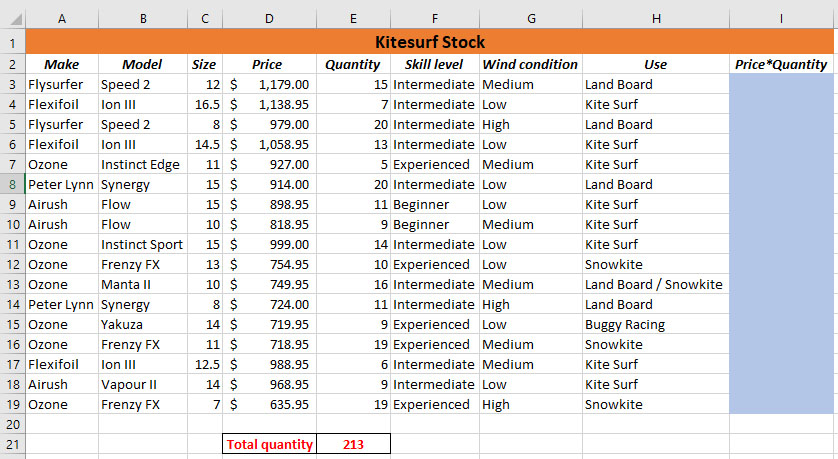
- The spreadsheet model describes data about Kitesurf stock.
- There are 9 columns, A:I
- There are 17 rows of data, rows 3:19
- Row 1 has merged all of the cells in the range A1:I1. The title is aligned in the center. The background color is orange.
- Some cells contain numbers eg cell C8.
- Some cells contain text eg cell F14.
- Cell E21 contains a calculation, the sum of every value in the range E3:E19.
- The data in column D is formatted as a currency to 2 decimal places.
Task
If you are using Google Sheets, use this sheet.
If you require a csv file to get started, download this one.
Using the above image as a guide:
Open the spreadsheet model. Note, some of the data may be different from the image above.
Enter the following data into row 18.

Insert a new column between column D and column E. Give the new column a title of Quantity.
In cell E2, type =randbetween(1,20). What a cool function :)
Copy down this function by dragging the handle in cell E2. Copy down to cell E18.
Format data in the Price column as US dollars to 2 decimal places.
In cell I1, type a column title of Order Price
In cell I2, calculate the Price multiplied by the Quantity.
Copy down the formula in cell I2 for every row of data in column I.
In cell I19, use the sum function to calculate the total price of all orders in column I.
Insert a new row at the top of the model. Then, merge all cells in the range A1:I1. Type Kiteboard Orders and format as follows:
- Alignment: center
- Background: orange
- Font-size: 24point
- Font: Calibri
Make sure all data in your spreadsheet model is visible.

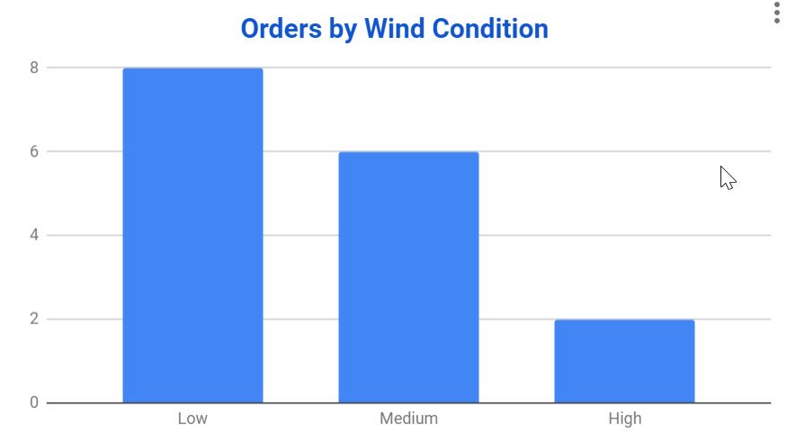
Can you make a bar chart which shows how many Low, Medium amd High Wind Condition models were ordered? It should look like (your data might be different):
Research 1
Can you figure out how to create a drop-down list in the size column? It should look like this and be in every cell in the size column:
Can you figure out how to create a drop-down list in the size column? It should look like this and be in every cell in the size column:
Research 2
Can you figure out how to create conditional formatting in the Price column? If the price is less than $800, the cell background color is red.
Can you figure out how to create conditional formatting in the Price column? If the price is less than $800, the cell background color is red.
Submit your final spreadsheet file as instructed.
Food For Thought
Today we generated some random numbers using the randbetween function. In the next section, we will be introduced to some more functions that do calculating for us!



Homework
Tags
spreadsheet data csv model merge insert row format currency column range decimal places cell reference